10. 타이타닉 생존자 예측[Decision tree 와 Randomforest 비교하기]
![10. 타이타닉 생존자 예측[Decision tree 와 Randomforest 비교하기]](https://github.com/HwangToeMat/HwangToeMat.github.io/blob/master/assets/img/thumbnail/dwp-13.png?raw=true)
타이타닉 생존자 예측[Decision tree 와 Randomforest 비교하기]
import pandas as pd
import numpy as np
import sys
Problem definition
Using data from passengers on the Titanic, try to find survival rates based on the characteristics of passengers.
Data definition
Data explanation
survival : Survival [0 = No, 1 = Yes]
pclass : Ticket class [1 = 1st(Upper), 2 = 2nd(Middle), 3 = 3rd(Lower)]
sex : Sex
Age : Age in years
sibsp : # of siblings / spouses aboard the Titanic
parch : # of parents / children aboard the Titanic
ticket : Ticket number
fare : Passenger fare
cabin : Cabin number
embarked : Port of Embarkation C = Cherbourg, Q = Queenstown, S = Southampton
train_f = pd.read_csv("../data/train.csv")
test_f = pd.read_csv("../data/test.csv")
test_a =pd.read_csv("../data/gender_submission.csv")
train_f.head()
| PassengerId | Survived | Pclass | Name | Sex | Age | SibSp | Parch | Ticket | Fare | Cabin | Embarked | |
|---|---|---|---|---|---|---|---|---|---|---|---|---|
| 0 | 1 | 0 | 3 | Braund, Mr. Owen Harris | male | 22.0 | 1 | 0 | A/5 21171 | 7.2500 | NaN | S |
| 1 | 2 | 1 | 1 | Cumings, Mrs. John Bradley (Florence Briggs Th... | female | 38.0 | 1 | 0 | PC 17599 | 71.2833 | C85 | C |
| 2 | 3 | 1 | 3 | Heikkinen, Miss. Laina | female | 26.0 | 0 | 0 | STON/O2. 3101282 | 7.9250 | NaN | S |
| 3 | 4 | 1 | 1 | Futrelle, Mrs. Jacques Heath (Lily May Peel) | female | 35.0 | 1 | 0 | 113803 | 53.1000 | C123 | S |
| 4 | 5 | 0 | 3 | Allen, Mr. William Henry | male | 35.0 | 0 | 0 | 373450 | 8.0500 | NaN | S |
test_f.head()
| PassengerId | Pclass | Name | Sex | Age | SibSp | Parch | Ticket | Fare | Cabin | Embarked | |
|---|---|---|---|---|---|---|---|---|---|---|---|
| 0 | 892 | 3 | Kelly, Mr. James | male | 34.5 | 0 | 0 | 330911 | 7.8292 | NaN | Q |
| 1 | 893 | 3 | Wilkes, Mrs. James (Ellen Needs) | female | 47.0 | 1 | 0 | 363272 | 7.0000 | NaN | S |
| 2 | 894 | 2 | Myles, Mr. Thomas Francis | male | 62.0 | 0 | 0 | 240276 | 9.6875 | NaN | Q |
| 3 | 895 | 3 | Wirz, Mr. Albert | male | 27.0 | 0 | 0 | 315154 | 8.6625 | NaN | S |
| 4 | 896 | 3 | Hirvonen, Mrs. Alexander (Helga E Lindqvist) | female | 22.0 | 1 | 1 | 3101298 | 12.2875 | NaN | S |
test_a.head()
| PassengerId | Survived | |
|---|---|---|
| 0 | 892 | 0 |
| 1 | 893 | 1 |
| 2 | 894 | 0 |
| 3 | 895 | 0 |
| 4 | 896 | 1 |
test_td = pd.concat([test_f, test_a], axis=1)
test_td = test_td.iloc[:,[0,12,1,2,3,4,5,6,7,8,9,10]]
titanic_df = pd.concat([train_f, test_td], axis=0)
titanic_df.head()
| PassengerId | Survived | Pclass | Name | Sex | Age | SibSp | Parch | Ticket | Fare | Cabin | Embarked | |
|---|---|---|---|---|---|---|---|---|---|---|---|---|
| 0 | 1 | 0 | 3 | Braund, Mr. Owen Harris | male | 22.0 | 1 | 0 | A/5 21171 | 7.2500 | NaN | S |
| 1 | 2 | 1 | 1 | Cumings, Mrs. John Bradley (Florence Briggs Th... | female | 38.0 | 1 | 0 | PC 17599 | 71.2833 | C85 | C |
| 2 | 3 | 1 | 3 | Heikkinen, Miss. Laina | female | 26.0 | 0 | 0 | STON/O2. 3101282 | 7.9250 | NaN | S |
| 3 | 4 | 1 | 1 | Futrelle, Mrs. Jacques Heath (Lily May Peel) | female | 35.0 | 1 | 0 | 113803 | 53.1000 | C123 | S |
| 4 | 5 | 0 | 3 | Allen, Mr. William Henry | male | 35.0 | 0 | 0 | 373450 | 8.0500 | NaN | S |
titanic_df.to_csv("../data/titanic_df.csv")
titanic_df = pd.read_csv("../data/titanic_df.csv")
# Check the summary of your current data
titanic_df.info()
<class 'pandas.core.frame.DataFrame'>
RangeIndex: 1309 entries, 0 to 1308
Data columns (total 13 columns):
Unnamed: 0     1309 non-null int64
PassengerId    1309 non-null int64
Survived       1309 non-null int64
Pclass         1309 non-null int64
Name           1309 non-null object
Sex            1309 non-null object
Age            1046 non-null float64
SibSp          1309 non-null int64
Parch          1309 non-null int64
Ticket         1309 non-null object
Fare           1308 non-null float64
Cabin          295 non-null object
Embarked       1307 non-null object
dtypes: float64(2), int64(6), object(5)
memory usage: 133.0+ KB
Data preprocessing
In fact, there is information that the accident first carried women and the elderly on lifeboats. Based on this information, we remove features from the data that would not have a significant impact on the survival forecast. Delete columns with too many null values and convert women to 0 and men to 1.
del titanic_df["Name"]
del titanic_df["Ticket"]
del titanic_df["Cabin"]
del titanic_df["Embarked"]
del titanic_df["Unnamed: 0"]
titanic_df.loc[titanic_df["Sex"] == "female",["Sex"]] = 0
titanic_df.loc[titanic_df["Sex"] == "male",["Sex"]] = 1
titanic_df = titanic_df.dropna()
titanic_df.head()
| PassengerId | Survived | Pclass | Sex | Age | SibSp | Parch | Fare | |
|---|---|---|---|---|---|---|---|---|
| 0 | 1 | 0 | 3 | 1 | 22.0 | 1 | 0 | 7.2500 |
| 1 | 2 | 1 | 1 | 0 | 38.0 | 1 | 0 | 71.2833 |
| 2 | 3 | 1 | 3 | 0 | 26.0 | 0 | 0 | 7.9250 |
| 3 | 4 | 1 | 1 | 0 | 35.0 | 1 | 0 | 53.1000 |
| 4 | 5 | 0 | 3 | 1 | 35.0 | 0 | 0 | 8.0500 |
titanic_df.describe()
| PassengerId | Survived | Pclass | Sex | Age | SibSp | Parch | Fare | |
|---|---|---|---|---|---|---|---|---|
| count | 1045.000000 | 1045.000000 | 1045.000000 | 1045.000000 | 1045.000000 | 1045.000000 | 1045.000000 | 1045.000000 |
| mean | 654.990431 | 0.399043 | 2.206699 | 0.628708 | 29.851837 | 0.503349 | 0.421053 | 36.686080 |
| std | 377.650551 | 0.489936 | 0.841542 | 0.483382 | 14.389194 | 0.912471 | 0.840052 | 55.732533 |
| min | 1.000000 | 0.000000 | 1.000000 | 0.000000 | 0.170000 | 0.000000 | 0.000000 | 0.000000 |
| 25% | 326.000000 | 0.000000 | 1.000000 | 0.000000 | 21.000000 | 0.000000 | 0.000000 | 8.050000 |
| 50% | 662.000000 | 0.000000 | 2.000000 | 1.000000 | 28.000000 | 0.000000 | 0.000000 | 15.750000 |
| 75% | 973.000000 | 1.000000 | 3.000000 | 1.000000 | 39.000000 | 1.000000 | 1.000000 | 35.500000 |
| max | 1307.000000 | 1.000000 | 3.000000 | 1.000000 | 80.000000 | 8.000000 | 6.000000 | 512.329200 |
- The summary of titanic_df shows that the survival rate is very low at 37.7%.
- Gender also shows that there are more males than females, and the average age group was lower than expected at 30.
Data Visualization
import matplotlib.pyplot as plt
import seaborn as sns
%matplotlib inline

f,ax=plt.subplots(1,2,figsize=(12,6))

titanic_df['Survived'].value_counts().plot.pie(explode=[0,0.1],autopct='%1.2f%%',ax=ax[0])
ax[0].set_title('Survived')
ax[0].set_ylabel('')

sns.countplot('Survived',data=titanic_df,ax=ax[1])
ax[1].set_title('Survived')
plt.show()
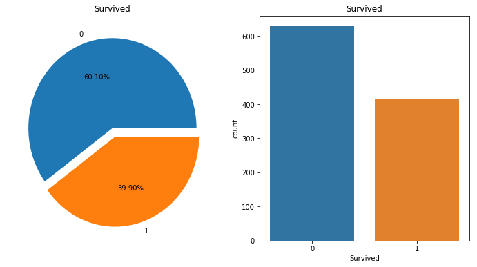
- Blue indicates death and orange indicates survivors.
plt.figure(figsize=[12,4])
plt.subplot(121)
sns.barplot('Pclass', 'Survived', data=titanic_df)
plt.subplot(122)
sns.countplot('Sex',hue='Survived',data=titanic_df)
plt.show()
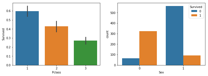
Comparing the survival rate by seat rating, one can see that the expensive seat has higher survival rate.
If you look at the graph on the right, it shows female deaths, female survivors, male deaths, and male survivors from the left. And we can see survival rate of female is much higher than male.
ax = titanic_df["Age"].hist(bins=15, color='teal', alpha=0.8)
ax.set(xlabel='Age', ylabel='Count')
plt.show()
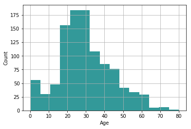
- The age distribution of passengers shows that they are concentrated in their 20s and 30s.
f,ax = plt.subplots(figsize=(12,6))
g = sns.kdeplot(titanic_df["Age"][(titanic_df["Survived"] == 0) & (titanic_df["Age"].notnull())],
                ax = ax, color="Blue", shade = True)
g = sns.kdeplot(titanic_df["Age"][(titanic_df["Survived"] == 1) & (titanic_df["Age"].notnull())],
                ax =g, color="Green", shade= True)
g.set_xlabel("Age")
g.set_ylabel("Frequency")
g = g.legend(["Not Survived","Survived"])
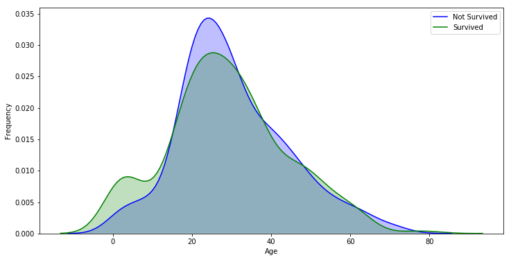
The most important part of this graph comparing survival rate and age is the green section, which represents a high percentage of survivors, and the purple section, which represents a high percentage of deaths.
Age under 17 group have a very high survival rate compared to other age groups.
Age between 17~35 group have a very high death rate compared to other age groups.
By analyzing the overall data, one can see that the younger , female and more expensive class of seats have higher survival rate. If we don’t think about class of seats, people tried to protect the weak first in the accident.
Data Division
# The train_test_split of sklearn makes it easy to divide data into a single line.
from sklearn.model_selection import train_test_split

train, test = train_test_split(titanic_df, test_size=0.2)
import pickle
with open('../data/fifa_train.pkl', 'wb') as train_df:
    pickle.dump(train, train_df)

with open('../data/fifa_test.pkl', 'wb') as test_df:
    pickle.dump(test, test_df)
with open('../data/fifa_train.pkl', 'rb') as train_df:
    train = pickle.load(train_df)

with open('../data/fifa_test.pkl', 'rb') as test_df:
    test = pickle.load(test_df)
Setting Optimal Parameters for a Model
We can deduce these values(max_depth, min_samples_split,mins_samples_leaf, random_state) through repetition.
from sklearn import tree
from sklearn import preprocessing
X_train = train[['Pclass', 'Sex', 'Age', 'SibSp', 'Parch', 'Fare']]
y_train = train[['Survived']]

X_test = test[['Pclass', 'Sex', 'Age', 'SibSp', 'Parch', 'Fare']]
y_test = test[['Survived']]
depth = list(range(1,100,5))
sample_split = list(range(2,100,5))
sample_leaf = list(range(2,100,5))
random_state = list(range(1,100,5))
clf_list = []
for i in depth:
    for j in sample_split:
        for k in sample_leaf:
            for l in random_state:
                clf_list.append(tree.DecisionTreeClassifier(max_depth=i,
                                  min_samples_split=j,
                                  min_samples_leaf=k,
                                  random_state=l).fit(X_train, y_train))
clf_list[-5:]
[DecisionTreeClassifier(class_weight=None, criterion='gini', max_depth=96,
             max_features=None, max_leaf_nodes=None,
             min_impurity_decrease=0.0, min_impurity_split=None,
             min_samples_leaf=97, min_samples_split=97,
             min_weight_fraction_leaf=0.0, presort=False, random_state=96,
             splitter='best')]
from sklearn.metrics import accuracy_score
accuracy_score_list = {}
for clf in clf_list:
    pred = clf.predict(X_test)
    accuracy_score_list[clf] = accuracy_score(y_test, pred)
len(accuracy_score_list)
160000
Choose the optimal clf with the highest accuracy among the 160,000 clf values.
max_accuracy = max(list(accuracy_score_list.values()))
best_clf = list(accuracy_score_list.keys())[list(accuracy_score_list.values()).index(max_accuracy)]
best_clf
DecisionTreeClassifier(class_weight=None, criterion='gini', max_depth=6,
            max_features=None, max_leaf_nodes=None,
            min_impurity_decrease=0.0, min_impurity_split=None,
            min_samples_leaf=2, min_samples_split=52,
            min_weight_fraction_leaf=0.0, presort=False, random_state=1,
            splitter='best')
Model test
pred = best_clf.predict(X_test)
Check the accuracy of the model prediction.
print("accuracy : " + str( accuracy_score(y_test, pred)) )
accuracy : 0.8325358851674641
Compare the actual and predicted values.
comparison = pd.DataFrame({'prediction':pred, 'ground_truth':y_test["Survived"]})
comparison
| prediction | ground_truth | |
|---|---|---|
| 167 | 0 | 0 |
| 900 | 0 | 0 |
| 345 | 1 | 1 |
| 369 | 1 | 1 |
| 645 | 0 | 1 |
| 69 | 0 | 0 |
| 463 | 0 | 0 |
| 943 | 1 | 1 |
| 1084 | 0 | 0 |
| 684 | 0 | 0 |
| 521 | 0 | 0 |
| 220 | 0 | 1 |
209 rows × 2 columns
Decision tree Visualization
import os
os.environ["PATH"] += os.pathsep + 'C:/Program Files (x86)/Graphviz2.38/bin/'
import graphviz
dot_data = tree.export_graphviz(best_clf, out_file=None)
graph = graphviz.Source(dot_data)
graph.render("titanic survived")

dot_data = tree.export_graphviz(best_clf, out_file=None,
                         feature_names=['Pclass', 'Sex', 'Age', 'SibSp', 'Parch', 'Fare'],
                         class_names=['Not Survived', 'Survived'],
                         filled=True, rounded=True,
                         special_characters=True)
graph = graphviz.Source(dot_data)
graph
Setting Optimal Parameters for Randomforest
from sklearn import datasets
from sklearn import tree
from sklearn.ensemble import RandomForestClassifier
from sklearn.model_selection import cross_val_score
if not sys.warnoptions:
    import warnings
    warnings.simplefilter("ignore")
estimators = list(range(1,200))
clf_list2 = []
for i in estimators:
    clf_list2.append(RandomForestClassifier(n_estimators=i).fit(X_train, y_train))
clf_list2[-5:]
[RandomForestClassifier(bootstrap=True, class_weight=None, criterion='gini',
             max_depth=None, max_features='auto', max_leaf_nodes=None,
             min_impurity_decrease=0.0, min_impurity_split=None,
             min_samples_leaf=1, min_samples_split=2,
             min_weight_fraction_leaf=0.0, n_estimators=199, n_jobs=1,
             oob_score=False, random_state=None, verbose=0,
             warm_start=False)]
from sklearn.metrics import accuracy_score
accuracy_score_list2 = {}
for clf in clf_list2:
    pred2 = clf.predict(X_test)
    accuracy_score_list2[clf] = accuracy_score(y_test, pred2)
len(accuracy_score_list2)
199
Choose the optimal clf with the highest accuracy among the 199 clf values.
max_accuracy2 = max(list(accuracy_score_list2.values()))
best_clf2 = list(accuracy_score_list2.keys())[list(accuracy_score_list2.values()).index(max_accuracy2)]
best_clf2
RandomForestClassifier(bootstrap=True, class_weight=None, criterion='gini',
            max_depth=None, max_features='auto', max_leaf_nodes=None,
            min_impurity_decrease=0.0, min_impurity_split=None,
            min_samples_leaf=1, min_samples_split=2,
            min_weight_fraction_leaf=0.0, n_estimators=29, n_jobs=1,
            oob_score=False, random_state=None, verbose=0,
            warm_start=False)
Randomforest Test
pred2 = best_clf2.predict(X_test)
Check the accuracy of the model prediction.
print("accuracy : " + str( accuracy_score(y_test, pred2)) )
accuracy : 0.8373205741626795
Compare the actual and predicted values.
comparison2 = pd.DataFrame({'prediction':pred2, 'ground_truth':y_test["Survived"]})
comparison2
| prediction | ground_truth | |
|---|---|---|
| 167 | 0 | 0 |
| 900 | 0 | 0 |
| 345 | 1 | 1 |
| 369 | 1 | 1 |
| 645 | 1 | 1 |
| 69 | 0 | 0 |
| 463 | 0 | 0 |
| 943 | 1 | 1 |
| 1084 | 0 | 0 |
| 684 | 0 | 0 |
| 521 | 0 | 0 |
| 220 | 0 | 1 |
209 rows × 2 columns
Cross_Validation
def cross_validation(classifier,features, labels):
    cv_scores = []

    for i in range(10):
        scores = cross_val_score(classifier, features, labels, cv=10, scoring='accuracy')
        cv_scores.append(scores.mean())

    return cv_scores
dt_cv_scores = cross_validation(best_clf, X_test, y_test)
if not sys.warnoptions:
    import warnings
    warnings.simplefilter("ignore")
rf_cv_scores = cross_validation(best_clf2, X_test, y_test)
Randomforest VS Decision tree
cv_list = [
            ['random_forest',rf_cv_scores],
            ['decision_tree',dt_cv_scores],
          ]
df = pd.DataFrame.from_items(cv_list)
df.plot()
<matplotlib.axes._subplots.AxesSubplot at 0x1ad431ac240>
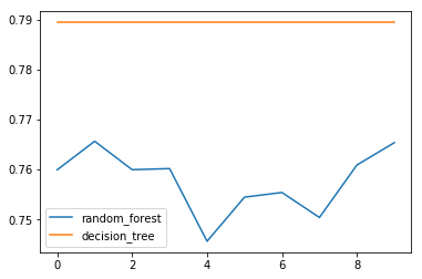
Accuracy of Decision Tree
np.mean(dt_cv_scores)
0.7894372294372294
Accuracy of Randomforest
np.mean(rf_cv_scores)
0.7577835497835498
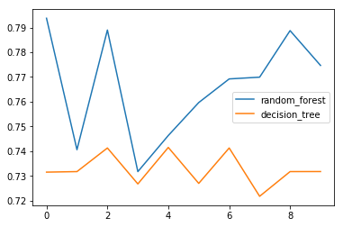
conclusion
In fact, we need to get better results from the random forest model..
However, in this report, the two models were obtained repeatedly to improve the predictability of test data while adjusting all the detailed figures.
In short, the above result is that there is a probability of being overfit.
Therefore, if you do not adjust the detailed figure and set it to the auto, results are as shown in the graph below.
cv_list = [
            ['random_forest',cross_validation(RandomForestClassifier(), X_test, y_test)],
            ['decision_tree',cross_validation(tree.DecisionTreeClassifier(), X_test, y_test)],
          ]
df = pd.DataFrame.from_items(cv_list)
df.plot()
<matplotlib.axes._subplots.AxesSubplot at 0x1ad5d9bf860>
etc..
The autosklearn package is said to be a way to obtain appropriate parameter values for different models. I would like to try autosklearn in the next report.